How to Properly Apply Dropout on Recurrent Neural Network?
Overview
Dropout is a useful tool for regularizing neural network, but applying it on Recurrent Neural Network could be very tricky! This blogpost would introduce 3 dropout techniques that are empirically effective in training Recurrent Neural Network for language models.
The techniques are originally introduced in a paper by Stephen Merity in 2017. Besides the dropout techniques, the paper also introduce a lot of additional regularization techniques such as ASG optimization, activation regularization and temporal activation regularization.
Since then the techniques have been widely used for training language models with RNN. In particular, FastAI community included the whole AWD-LSTM network in its library and further develop a transfer learning framework called ULMFit that is built on top of AWD-LSTM network.
I recently have a leisure time to read through the original paper and find that the dropout techniques include a lot of details that could be hard to digest. Therefore, this blogpost aims to illustrate the dropout techniques augmented with visual diagrams. I hope it could help the readers more easily understand the dropout techniques introduced in the paper.
The 3 dropout techniques I would introduce are (1) dropout on word embedding, (2) dropout on hidden state, and (3) dropout on hidden-to-hidden weight matrix. I would firstly give you a brief introduction to word embedding and recurrent layer. After that, I will highlight each dropout technique one by one.
What is Dropout?
Before diving into the techniques, let’s briefly review what dropout is. Dropout is a famous weapon for fighting against model overfitting. In essence, dropout is a binary mask applied on a layer (usually the layer applied is an activation layer). It randomly zeroes out each activation unit with a specified chance. By doing so it could effectively discourage model from relying on a small subset of neurons but instead utilize more of its neurons, and hence boosting the generalization power of a model.
Dropout typically mask each activation unit independently with a specified probability. This setting has gained a dominant success in Convolution Neural Network but failed miserably in Recurrent Neural Network because such independency seriously hurts RNN from learning long-term dependency relationship. The various dropout techniques I introduce below are essentially to impose different dependency structure on the dropout mask so as to effectively regulate RNN.
insert CNN dropout visuals
A Briefly Introduction Word Embedding
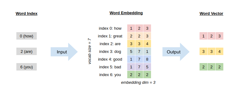
In language model, we usually have a fixed set of vocabulary and we represent each word by a vector. Word embedding is essentially a weight matrix storing all these vectors. Just imagine a word embedding is a compat storage with all vectors vertically packed so that its row is the vocabulary size and its col is the dimension of the vecotr. You could retrieve the vector of a word by its corresponding index.
Technique 1: Dropout on Word Embedding
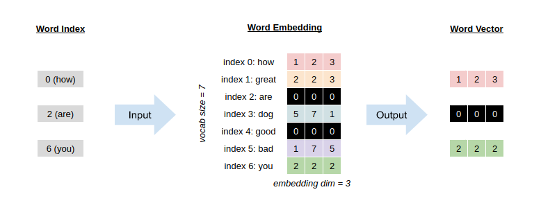
Applying dropout on word embedding is anologous to disappearing some words from a vocabulary. To achieve such effect, we could randomly select some words (indexes) from the vocabulary and completely zero out their vectors. Technically, it is equivalent to randomly masking out some rows of the word embedding weight matrix.
To minimize the operation, such dropout mask only updates once for each mini-batch and it is applied on the word embedding before feed-forward pass. Another details is that the dropout mask on word embedding is not a binary mask. Instead, it scales non-masked weight by a factor of $1/(1-p)$ where $p$ is the probability that a word to be masked out. In other words, a higher $p$ leads to a larger scaling factor on non-masked weight.
A Brief Introduction to Recurrent Layer
Recurrent Neural Network is a composition of recurrent layer(s). There are many variants of RNN and each variant has its unique design of recurrent layer. For example, one of its variant Long Short Term Memory Network (LSTM) introduces forget, input, cell and output gates in its recurrent layer for better performance. To avoid dwelling into those complexity, I will mainly focus on vanilla recurrent layer, but keep in mind that the dropout principles introduced here can be applied to all RNN variants. Also note that the notations used below mainly follow PyTorch documentation.
Recurrent layer is designed to handle sequence data. In contrast to image data, sequence data usually have serial dependency and they have variable length. Recurrent layer processes sequence data across timestep using its shared parameters. Such design is an efficient structure for model parameterization (less parameters to be learned) and capturing essential dependency (memory).
In order to store the essential memory from the preceding timesteps, recurrent layer introduces an activation layer called hidden state $\bold{h_{t-1}}$. At each time step $t$, a recurrent layer receives input vector at current timestep $\bold{x_{t}}$ and hidden state at preceding timestep $\bold{h_{t-1}}$ to generate hidden state at current timestep $\bold{h_t}$. Finally, $\bold{h_t}$ is passed to 2 places - one for output of the recurrent layer and another for the recurrent input of the recurrent layer in the next timestep.
insert RNN diagram overview
Note that $\bold{x_{t}}$ and $\bold{h_{t-1}}$ often have different dimension. To abbreviate, lets denote the input vector’s dimension as input_size and hidden state’s dimension as hidden_size. Mathematically underneath the hood of the recurrent layer, $\bold{x_{t}}$ and $\bold{h_{t-1}}$ are undergoing the following transformation to get $\bold{h_t}$:
\[\bold{h\_{t}} = f(\bold{W\_{ih} x_{t} + W\_{hh} h\_{t-1} + b\_{ih} + b\_{hh}})\]We call $\bold{W_{ih}}$ as input-to-hidden weight matrix because it helps transform an input vector into a vector of size hidden_size. By the same token, we call $\bold{W_{hh}}$ as hidden-to-hidden weight matrix. Activation function $f$ is usually a hyperbolic tangent function $tanh$. Lastly, $\bold{b_{ih}}$ and $\bold{b_{hh}}$ are bias terms.
insert inner mechanism of Recurrent layer
The above overview should suffice to introduce the remaining 2 types of dropout techniques for regulating recurrent layers.
Technique 2: Dropout on Hidden State
An intuitive way to regulate recurrent layer is to apply dropout on hidden state. However, there are several caveats we need to notice when doing so:
- Only hidden state for output has dropout applied, hidden state for next timestep is free from dropout
- For different samples in a mini-batch, they should have different dropout masks applied on their hidden state
- For different timesteps of a given sample, the same dropout mask must be applied on its hidden state
- In case of multiple recurrent layers, different dropout masks are applied on different hidden states for a given sample
- In case of multiple recurrent layers, the hidden state output from the final layer does not have dropout applied
Similar to dropout on word embedding, the dropout masks on hidden state only update once for each mini-batch, before feed-forward pass.
Here are some simple diagrams to illustrate the above details:
several diagrams to illustrate dropout on hidden states
Technique 3: Dropout on Hidden-to-Hidden Weight Matrix
There are empirical studies showing that overfitting easily appear in recurrent connection of a recurrent layer. To combat such overfitting, we could apply dropout on hidden-to-hidden weight matrix. Such dropout could mitigate the chance that the overfitting in one timestep would significantly propagate to the next timestep. Similar to the above, there are a few caveats to note on its details:
- Once the dropout mask is applied on the hidden-to-hidden weight matrix, the mask is locked for all samples and all timesteps in a mini-batch
- In case of multiple recurrent layers, different dropout masks are applied on hidden-to-hidden weight matrix of different recurrent layers
Again, the dropout mask on hidden-to-hidden weight matrix is only update once for each mini-batch, before feed-forward pass. In the original paper, authors mention that applying dropout on input-to-hidden weight matrix could also help, but applying so on hidden-to-hidden weight matrix already suffice.
Below diagrams illustrate how dropout on hidden-to-hidden weight matrix works in details:
diagrams
Putting All Dropout Techniques Together
The diagrams below best summarize how it looks like when all dropout techniques are applied on a RNN of multiple recurrent layers:
diagrams
Closing Remark
At last, I hope this article could help clear most of the subtleties in the dropout schemes from AWD-LSTM Network. Finally, I hope you enjoy this blogpost!