Paper Summary: "PlenOctrees for Real-time Rendering of Neural Radiance Fields"
NeRF is powerful for learning a 3D scene's representation generalizable to novel views, but it suffers from slow rendering speed. This paper proposes a variant called NeRF-SH and a data structure for caching called PlenOctree. When applied together it drives significant speedup on rendering with comparable rendering quality against vanilla NeRF.
- 1. Motivations
- 2. Introduction to Spherical Harmonics
- 3.1. NeRF-SH: Linking Spherical Harmonics to NeRF
- 3.2. NeRF-SH: Training with Sparsity Loss
- 4.1. Conversion to PlenOctree
- 4.2. Rendering with PlenOctree
- 4.3. Fine-tuning PlenOctree
- 5. Experimental Results
- 6. Limitations
- 7. References
1. Motivations
Neural Radiance Field (NeRF) has gained traction in academia thanks to its power to render novel 2D views of a 3D scene trained on the posed images. However NeRF’s rendering speed is noticeably slow. Without a GPU accelerator, it could easily take more than 1 minute to render a 2D view. Such drawback blocks its application on latency-sensitive domain.
It is slow becaues numerous network calls have to be made for rendering even one single pixel. The authors of this paper propose the following to address this issue and achieves a significant speedup:
- Invent an efficient data structure called PlenOctrees to spatially cache the outputs from a trained NeRF
- Introduce a variant of NeRF (NeRF-SH) that is easily convertible into PlenOctree representation
2. Introduction to Spherical Harmonics
Spherical Harmonics (SH) is a critical concept behind their proposal. Shperical Harmonics is a collections of spherical functions used to describe the surface of some special spheres.
Technically, each of the function receives a direction in 3D space, parametrised as $(\theta, \phi)$, as an input and the absolute value of its output (output is a complex number) tells you the associated surface’s distance from the origin. The functions are usually annotated as $Y_{l}^{m}(\theta, \phi)$ where $m$ and $l$ determines the shape of the sphere to be described.
Below visualise some instances of the shperical surfaces:

In the same sprit that some functions can be decomposed into polynomials, and that any periodic functions can be decomposed into Fourier Series, Spherical Harmonics are powerful enough to express any spherical function when composed together properly.
Additionally it provides a compact way to represent any spherical functions. We only need to book keep the coefficients for each SH function and then we can recover the target spherical function at any input (details in next session).
How could we apply this concept to NeRF? Recall that NeRF describes the geometry (i.e. density $\sigma$) and appearance (i.e. RGB colour $\bold{c}$) of any 3D point $\bold{x}$ in a 3D scene at any viewing direction $\bold{d}$. While a 3D point’s density is invariant of your viewing direction, its colour varies with your viewing angle. Therefore, we can treat the colour exactly like spherical function, except that we need 3 independent real-valued spherical functions to do so because we need 3 channels (red, green and blue) to describe a RGB colour.
3.1. NeRF-SH: Linking Spherical Harmonics to NeRF
The authors propose NeRF-SH that models a 3D point’s colour as spherical fucntions. NeRF-SH receives a 3D point $\bold{x}$ as input and predicts its density $\sigma$ the same way as vanilla NeRF does. But instead of predicting its RGB colour for a single viewing direction, NeRF-SH predicts spherical functions that describes the colours at all viewing direction. This modification helps factor out viewing direction from the network input. It enables a space-efficient way to spatially cache the colours predicted by the network (into a PlenOctree structure).

We can compactly express a spherical function as coefficients of Spherical Harmonics $(k_{l}^{m})_{l:0\leq l \leq l_{max}}^{m: -l \leq m \leq l}$, where $k_{l}^{m}$ is 3-dimensional for describing the 3 channels of RGB colour.
Once we yield the coefficients $(k_{l}^{m})_{l:0\leq l \leq l_{max}}^{m: -l \leq m \leq l}$, we could easily render the colour at any viewing direction by a sum of Spherical Harmonics $\bold{Y}_{l}^{m}(\theta, \phi)$ weighted by their associated $k_{l}^{m}$, followed by a sigmoid transformation $S(.)$:

We can neatly summarize the pipeline for training NeRF-SH with a diagram extracted from the paper.

3.2. NeRF-SH: Training with Sparsity Loss
There is an additional caveat for the training: when solely supervised by standard reconstruction loss during training, NeRF-SH tends to predict arbitrary geometry on unused region. Although it doesn’t hurt the rendering quality but it occupies a lot of redundant space when NeRF-SH is converted into PlenOctree.
To encourage NeRF-SH to predict unused region to be empty, a sparsity loss is additionally enforced. To evaluate the loss, we uniformly sample $K$ points within a bounding box and consider their associated densities $\sigma_{k}$. High density leads to high sparsity loss.

With sparsity loss enforced, the unused region can be effectively pruned away from PlenOctree thanks to their negligible densities. As a result, it leads to a tighter bound on a 3D scene and hence a higher spatial resolution on PlenOctree representation (because voxel cells are mostly distributed to the important region).

4.1. Conversion to PlenOctree
Once NeRF-SH is trained, we can easily converted it into a PlenOctree representation with the following procedures:
- Evaluation: Sample uniformly spaced 3D grid points and evaluate their density $\sigma$ with the trained NeRF-SH.
- Filtering: Partition the grid points into different voxel cells. Render all training views and keep track of the maximum ray weight $1-exp(-\sigma_{i} \delta_{i})$ in each voxel cell, where $\delta_{i}$ is the distance between sample points along a ray (more details in next session). Cell with low ray weight implies it is likely an empty space with negligible contribution to any training views so we can safely prune them.
- Sampling: To determine the SH coefficients for each voxel cell, we randomly sample 256 points within a voxel cells and take an average of their associated SH coefficients.
4.2. Rendering with PlenOctree
With the converted PlenOctree, we could easily achieve blazingly fast rendering speed with the following procedures:
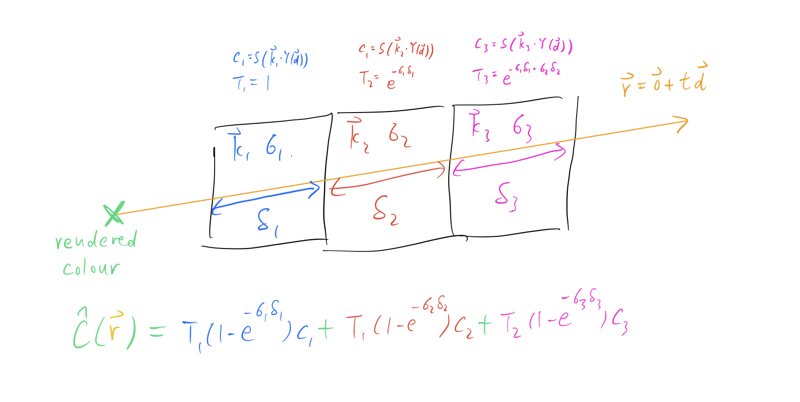
- Cast a ray $\bold{r}$ from the pixel to be rendered into the PlenOctree and consider all voxel cells that intersect with the ray.
- Segment the ray by voxel boundaries. Consider the lengths of each segments as ${\delta_{i}}_{i=1}^{N}$ and look up their associated density ${ \sigma_{i} }_{i=1}^{N}$ and SH coefficients ${ \bold{k_{i}} }_{i=1}^{N}$ from each voxel cell. Colour of each segment ${ c_{i} }_{i=1}^N$ can be found with the spherical functions represented by the SH coefficients.
- With the above quantities, apply standard volumetric rendering formula to render colour $\hat{C}(\bold{r})$ at the target pixel.
- We could achieve further speedup by early stopping the ray when its accumulated transmittance $T_{i}$ is too low. The accumulated transmittance indicates the chance that the ray can pass through the first segment up to the target segments without being blocked. Points with low accumulated transmittance have negligible impact to the rendered colour so we could safely skip them.

The whole process is similar to that of NeRF except PlenOctree makes use of cache from its voxel cells so it can achieve significant speedup comparing against a standard NeRF.
We can summarise the rendering process with a diagram below. $Y(.)$ is the SH functions as a vector and $\bold{k}_{i}$ are the SH coefficients associated to the $i$-th voxel cell. $c_{i}$ is its associated colour and the formula is no different from what we discussed before.
4.3. Fine-tuning PlenOctree
Since the rendering process with PlenOctree is done by standard volumetric rendering, the operation is differentiable. Therefore, we could apply stochastic gradient descent to fine-tune the PlenOctree representation. Empirical studies show that additional fine-tuning on PlenOctree could lead to significant improvement on rendering quality.
While in principle it is feasible to train a PlenOctree representation from scratch, it usually takes much more time to converge. A trained NeRF-SH gives PlenOctree a good prior of geometry and appearance to learn from.
We can neatly summarised the pipeline for yielding a PlenOctree representation with the following diagram extracted from the paper.

5. Experimental Results
The authors compares both the rendering speed and quality between their approach (NeRF-SH + PlenOctree) and existing models. The rendering speed is measured by Frames per Second (FPS) and the rendering quality is measured by Peak Signal-to-Noise Ratio (PSNR).
They experimented their approach with different settings (e.g. higher filtering threshold on accumulated transmittance, reduce grid size to 256) and found that a few of its settings (i.e. Ours-1.9G) achieved better PSNR and 3000x faster FPS against vanilla NeRF!

6. Limitations
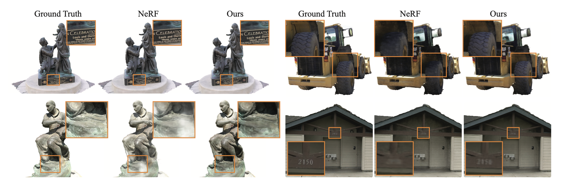
While NeRF-SH and PlenOctree achieves amazing rendering speed with comparable rendering quality against standard NeRF, it has several trade-offs.
On one hand, it has larger memory footprint than a standard NeRF. A NeRF model is typically light-weighted with roughly ~10 MB. However, a PlenOctree representation could easily take up to ~2 GB because it caches density and SH coefficients in each voxel cell.
On the other hand, it creates noticeable artifact when you zoom in the scene because it partitions a continuous 3D space into discrete voxel cells. The resolution is inevitably sacraficed.
