Paper Summary: "NeRF++: Analyzing and Improving Neural Radiance Fields"
Standard NeRF fails to respect the fidelity of an unbounded scene because its assumptions are too restrictive for scene where objects can be anywhere and background is indispensable. NeRF++ addresses the issue by a smart parameterization of foreground and background with 2 separate networks.
- 1. Motivations
- 2.1. How Could NeRF Possibly Learn So Well?
- 2.2. The Answer Lies On Its Design!
- 3.1. NeRF Shortcoming for Modelling Unbounded Scene
- 3.2. Parameterising Background as an Inverted Sphere
- 3.3. Finding $(x’, y’, z’)$ from $1/r$
- 4. Experimental Results
- 5. Limitations
- 6. References
1. Motivations
Thanks to over-parameterization, Neural Radiance Field (NeRF) has strong expressive freedom to describe a 3D scene’s geometry and its radiance. How is it possible to escape from numerous wrong solutions and converge to a correct one?
This is a question captivating authors’ attention. It turns out the anwser lies on some choices of design on NeRF’s structure which implicitly impose a form of regularization on its learning. (I personally find this part irrelevant to their main proposal, but it does offer me a new perspective on NeRF).
Despite such amazing capacity, NeRF has difficulty to learn some kinds of scenes. Unbounded scene is one of them which the authors are trying to address. It has its unique challenges because its background is indispensable to render and objects can be anywhere in the scene.
Standard NeRF doesn’t work well for unbounded scenes because it encloses a scene by a finite volume where it draws samples for volumetric rendering. To address the problem, the authors propose NeRF++ to model foreground and background as 2 separate volumes.
2.1. How Could NeRF Possibly Learn So Well?
NeRF is a neural network which describes the geometry (i.e. density) and radiance (i.e. colour) of a 3D scene. By the law of Universal Approximation Theorem, network like this could approximate any continuous functions. With so much expressive freedom empowered by its design, NeRF could possibly go wrong in many ways to overfit to training set without generalizing to novel views, unless we have a dense set of training examples as strong supervision.
The authors did an experiment to illustrate the point. They forced NeRF to learn wrong geometry (i.e. surface of a unit sphere) while supervised its radiance on a set of posed views from lego scene. Despite the fact that its learned geometry is far from lego-like, it manged to explain well on views from training set. Not surprisingly the trained NeRF failed miserably to render any novel views from test set.

This study suggests that NeRF’s expressive capacity is clearly overpowered, to a degree that even if it screws up on geometry, it could still fit perfectly to the training views. The authors call this phenomenon “shape-radiance ambiguities”.
But unexpectedly many empirical studies show that NeRF could typically learn the correct geometry and radiance of a 3D scene. It is therefore captivating to ask: How on earth could NeRF learn so well in spite of so much freedom to go wrong?
2.2. The Answer Lies On Its Design!
It turns out the sanity of NeRF has been secretly safeguarded by some choices of design in its model structure, which implicitly serve as a form of regularisation against its learning. The role of these decisions on model was rarely discussed in previous literatures, and this paper finally takes the chance to reveal it.
The authors conjecture 2 possible decisions on NeRF’s model structure that drives it towards correct geometry and radiance at high chance:
1. Low-frequency Encoding on View Direction
One trick applied by original NeRF is to project both viewing direction $(\theta, \phi)$ and spatial coordinate $(x, y, z)$ into high dimensional space by positional encoding. The encoding is independently cast on each parameter. We could formalize the encoding as $\gamma^{L}(p)$, where $L$ is a hyper-parameter that controls the dimension of its output and input $p$ is bounded by $[-1, 1]$:
Note that $sin(2^{L-1}\pi p)$ or $cos(2^{L-1}\pi p)$ has higher frequency with increasing $L$, so higher $L$ does not only contribute to higher dimensional space but also higher frequency variation on the output. As a result, positional encoding is conducive for NeRF to learn high-frequency details of a scene. To illustrate the impact of positional encoding on rendering quality, Ankur Handa has made an excellent visual comparison:
This is a great blog that provides intuitive explanation of the positional encoding used in transformers https://t.co/x8Mse71ARP
— Ankur Handa (@ankurhandos) April 19, 2020
Unlike RNNs transformers do not have any notion of word order so this positional encoding helps in capturing the order of words in sequence. pic.twitter.com/2IKJMamNE5
Now comes the hidden details - viewing direction is encoded by $\gamma^{4}(p)$ while spatial coordinate is encoded by $\gamma^{10}(p)$. This implies that features encoded from viewing direction is not so sensitive to high frequency variation compared against that from spatial coordinate. This favors the view-dependent radiance to be smooth and of low frequency with respect to the change in viewing direction.
Incorrect geometry has to be compensated by high-frequency radiance to explain well on training samples. Such low-frequency encoding on viewing direction makes NeRF struggle on high-frequency radiance, and hence guide it towards correct geometry.
2. Viewing Direction Injected at the Near End of Network
The more layers an input feature has passed through, the more complex pattern it could expresse thanks to compounded compositions of non-linear transformations. While spatial coordinate is fed as an input at the beginning of the network, viewing direction is only appended at almost the end.
This limits the complexity that viewing direction could express as features. But on the flip side, it actually serves as a form of regularization to prevent the view-dependent radiance from going too wild.

3.1. NeRF Shortcoming for Modelling Unbounded Scene
Having said NeRF comes with regularization in its structure, it is not without its shortcomings. One issue that the authors is trying to address is its limitation to model unbounded scenes.
Previous studies typically experimented NeRF on bounded scenes that are properly controlled, where an object of interest is centered at a stage and the posed views are taken at roughly a fixed distance from the object. Synthetic Dataset is one of the typical benchmark datasets in point. Such controlled environment makes NeRF easier to learn the scene, but they are far from any representations of scenes we would encounter in real life.

In practice scenes are unbounded - there could be more than one object of interest and objects could be anywhere in the scene. In particular, background is an indispensable part of the scene so a model should preserve fidelity of both foreground and background in order to be representative of an unbounded scene.

All these conditions impose significant challenges to standard NeRF. It is caused by the setting that during volumetric rendering standard NeRF samples 3D points from a packed volume. It works well for controlled environment because we know where the object lies, but for unbounded scenes the volume is unlikely to capture most objects from background. The consequence is a blurry background thanks to insufficient sampling of objects from background.
One remedy is to extend the length of the interval in a hope to cover most objects for sampling, but doing so has several practical limitations. If we fix the number of samples per traced ray, the rendered would look blurry in overall because of insufficient samples assigned to both foreground and background. But if we increase the number of samples, it significantly ramps up the computational cost which makes both training and rendering much more time-consuming. On top of that, it would be numerically unstable to evaluate points at far distance from the viewer.
To validate the claim, the authors have shown from experiment that standard NeRF struggles to render views of high fidelity in an unbounded Truck scene.

3.2. Parameterising Background as an Inverted Sphere
The authors propose NeRF++ to address the issue. Its model structure is the same as standard NeRF, except that it segregates foreground and background of a scene into 2 separate networks:
- Inner NeRF learns the foreground enclosed by a volume of unit sphere centered at origin
- Outer NeRF learns the background enclosed by a volume of its complement (i.e. an inverted sphere).
With such segregation, volumetric rendering has to take into account constitutes from both foreground and background along a traced ray in order to render colour for a pixel $\bold{C}(\bold{r})$. If we denote $t’$ as the time that the traced ray crosses the boundary between the two volumes, its theoretical formulation can expressed as follows:
The former term is numerical rendering of foreground and the latter term is that of background.
One caveat that deviates NeRF++ from the above formula is that outer NeRF receives different inputs than inner NeRF. Same as standard NeRF, inner NeRF is parameterized to return density $\sigma_{in}(\bold{x})$ and colour $\bold{c}_{in}(\bold{x}, \bold{d})$ for a spatial coordinate $\bold{x}$ at viewing direction $\bold{d}$. However, outer NeRF is parameterized slightly different: instead of treating target coordinate $\bold{x}$ as input, it firsly projects $\bold{x}$ onto the unit sphere to yield coordinate $\bold{x’} = (x’, y’, z’)$. And then it takes $\bold{x’}$ and the inverse of target coordinate’s distance $1/r$ as input. As a result, its outputs are parameterized as $\sigma_{out}(\bold{x’}, 1/r)$ and $\bold{c}_{out}(\bold{x’}, 1/r, \bold{d})$.
I personally find such parameterization clever because it skillfully normalises an unbounded spatial coordinate to bounded quantities. Such normalisation helps network to learn the background scene more efficiently. In addition, transforming unbounded inputs to bounded ones help avoid numerical unstability in optimization.
3.3. Finding $(x’, y’, z’)$ from $1/r$
I think it is worth some space to explain how we could find $(x’, y’, z’)$ and $1/r$.
Let’s say we have a traced ray $\bold{r}(t) = \bold{o} + t \bold{d}$ marching from the inner volume through the outer volume. We start off by randomly sample $1/r$ from the interval $(0, 1)$. The value of $r$ (note that this $r$ is different from the traced ray $\bold{r}(t)$!) should determine the target coordinate $\bold{x}$ that we want: it is the point that lies on the traced ray at a distance of $r$ from the origin. With $\bold{x}$ we could therefore find its projection onto the unit sphere.
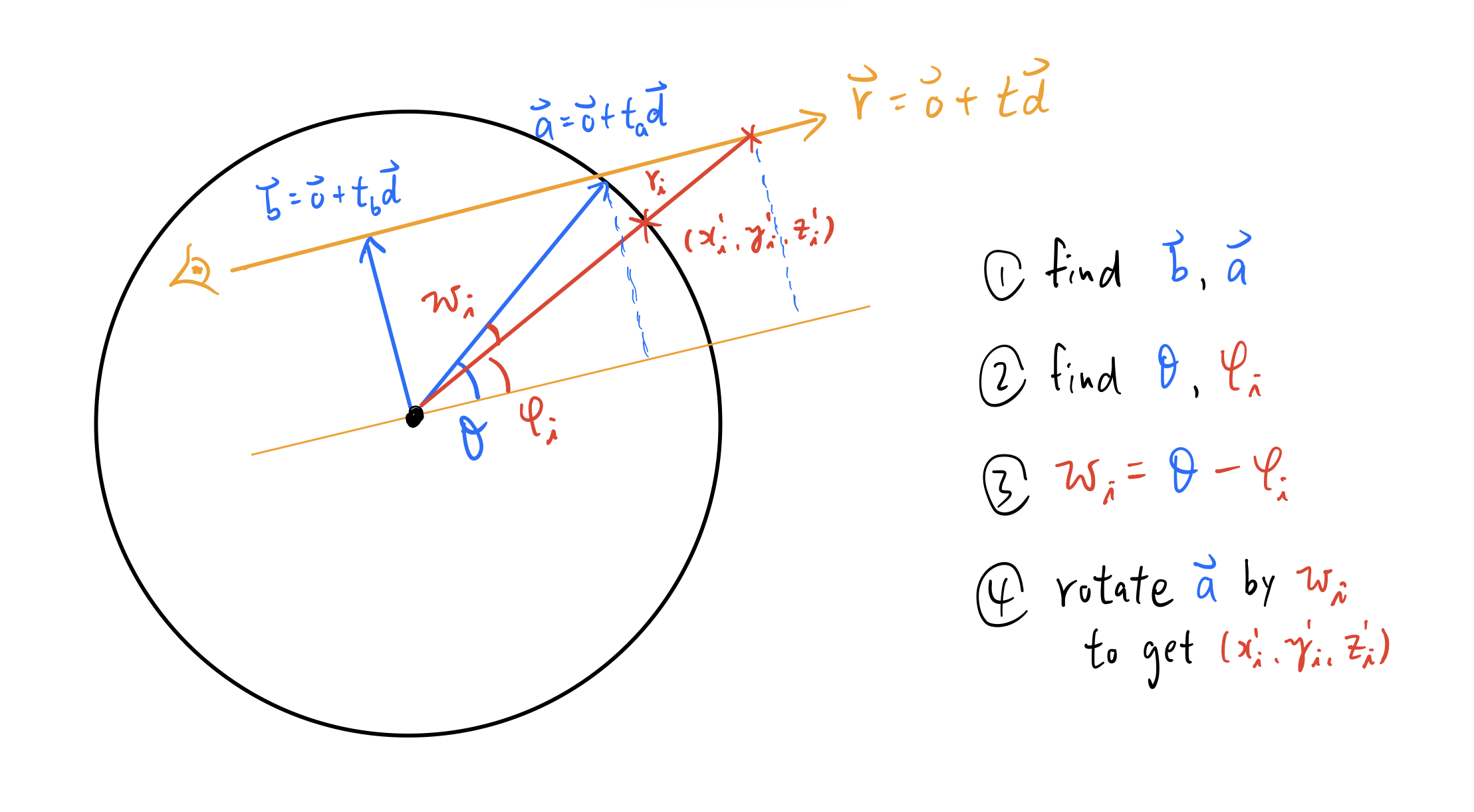
While the above intuition should work in principle, there is a simpler approach to find $(x’, y’, z’)$, as follows:
- Let $\bold{b} = \bold{o} + t_{b} \bold{d}$ to be the vector that is perpendicular to the traced ray. Find $\bold{b}$ by solving the equation $\bold{d} \cdot (\bold{o}+t_{b} \bold{d}) = 0$ for $t_{b}$
- Let $\bold{a} = \bold{o} + t_{a} \bold{d}$ to be the vector intersecting the unit sphere and the traced ray. Find $\bold{a}$ by solving the equation $\Vert \bold{o} + t_{a} \bold{d} \Vert = 1 $ for $t_{a}$
- Let $\theta$ be the angle between $\bold{a}$ and the traced ray. Find $\theta$ by solving $sin(\theta) = \Vert \bold{b} \Vert$
- Let $\phi$ be the angle between the target coordinate $\bold{x}$ and the traced ray. Find $\phi$ by solving $sin(\phi) = \Vert \bold{b} \Vert / r$
Finally we get $\omega = \theta - \phi$. This is the clockwise rotational angle along the plane $\bold{b} \times \bold{a}$ that we can apply to $\bold{a}$ in order to make it aligned to the target projection $(x’, y’, z’)$! One merit of this approach is that when $r$ is updated, we only need to simply update $\phi$ and $\omega$ in order to apply another round of angular rotation on $\bold{a}$!
The geometry of this approach can be neatly visualized below. Note that I draw the geometry in 2D (instead of 3D) just for the convenience of illustration:
4. Experimental Results
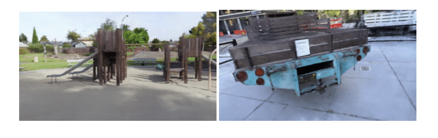
NeRF++ managed to render views that look sharp in both foreground and background. In comparison, background rendered by NeRF looks particularly blurry. Below are some experimental results for the scenes taken from Tanks and Temples benchmark dataset:

The diagram below shows that the proposed parameterisation done by NeRF++ has faithfully segregated foreground from background, without sacrificing the overall fidelities of the Truck scene.

Below are quantitative comparison on the same dataset. We can clearly notice that NeRF++ significantly outperforms NeRF for all scenes and all metrics.
As a remark, LPIPS stands for Learned Perceptual Image Patch Similarity which captures differences between image patches (lower means better) and SSIM stands for Structural Similarity, which captures perceptual similarity between 2 images.

5. Limitations
- Higher Computational Cost: NeRF++ is more costly on training and rendering than standard NeRF. It takes ~24 hours with 4 RTX 2080 Ti GPUs to train NeRF++ and ~30 seconds to render a single 1280x720 image.
- Ignorance to Photometric Effect: Though not a issue specific to NeRF++, it doesn’t take into account unexpected photometric effects such as auto-exposure, vignetting caused by a camera. These effects may contaminate the training samples because it leads to views of different colours even at the same pose, which breaks an assumption imposed on NeRF: same colour should be rendered at same pose.