Paper Summary: "BlockNeRF: Scalable Large Scene Neural View Synthesis"
NeRF has finally found its place in industrial application! BlockNeRF extends NeRF to reconstruct realistic city map at large scale. It effectively saves the expensive cost of data collection by simulating realistic driving views of diverse scenearios, accelerating the development of autonomous driving.
- 1. Motivations
- 2. An Overview of BlockNeRF’s Architecture
- 3. Orchestrating the Blocks
- 4. Results
- 5. Limitations
- 6. References
1. Motivations
BlockNeRF has recently taken the Twitter’s ML community by storm. Intrigued by its amazing demo of realistic driving views at different landmarks, I am hooked to read its paper.
Block-NeRF: Scalable Large Scene Neural View Synthesis
— AK (@_akhaliq) February 11, 2022
abs: https://t.co/xDa1bmJaCJ
project page: https://t.co/IQTnknxTuK pic.twitter.com/HX7cSx6Yh1
Jointly developed by Google and Waymo, BlockNeRF extends NeRF to reconstruct realistic city map at large scale. This is not the first work on scalable scenes with NeRF. To name a few, MegaNeRF reconstructs wild landscape with drone data, and CityNeRF reconstructs map in city scale. However, BlockNeRF is the first work applying NeRF on automonous driving.
How does BlockNeRF help with automonous driving? Automonous vehicles requires sheer volume of driving scenarios for training but collecting them first hand at scale is expensive. As an alternative, researchers actively explore the possibility to simulate realistic driving scenes with deep learning models. One proposal is to simulate scenes from a virtual world (just imagine the scenes you see in GTA). However, it is undesirable because the simulated scenes are neither representative to reality nor diverse. On the contrary, BlockNeRF is capable to simulate realistic driving scenes with huge variety.
2. An Overview of BlockNeRF’s Architecture
BlockNeRF is a variant of Neural Radiance Field network (aka NeRF). As a very brief introduction, NeRF learns to reconstruct a 3D scene from its 2D views and their associated viewpoints. We can treat a scene as a bounded volume and NeRF describes the density $\sigma$ and RGB colour $\bold{c}$ of any position in the space. Once trained, NeRF can project the 3D scene into 2D image at any viewpoints. It deploys a classical technique called volumetric rendering to render each pixel by tracing a ray from the viewpoint, through the pixel, to the scene.
I will highlight some key techniques by BlockNeRF, together with its architecture. Due to limited space, I will spare their nitty gritty details.
Below diagram best summarises BlockNeRF’s design and I will explain each component in the following sessions.
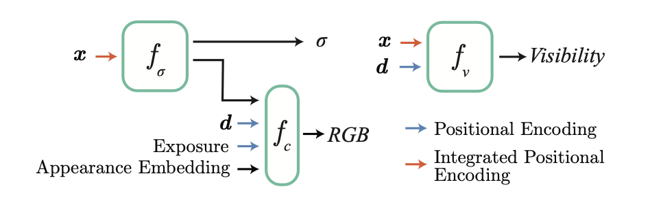
2.1. Segregating Sub-networks $f_{\sigma}$ and $f_{\bold{c}}$
BlockNeRF divides a gigantic scene into blocks and then conquer each block with an individual NeRF network. But unlike standard NeRF, it segregates the prediction of density and colour into 2 different sub-networks, namely $f_{\sigma}$ and $f_{\bold{c}}$.
2.1.1. Density Prediction by $f_{\sigma}$
The 1st sub-network $f_{\sigma}$ predicts the density $\sigma$ at position $\bold{x}$. The sub-network only requires position as input because geometry only depends on space. No matter how you view the same position at different angles or at varying lighting conditions, its geometry should be the same. Besides $\sigma$, the sub-network $f_{\sigma}$ spits out a high-dimensional embedding, to be consumed by the 2nd sub-network $f_{\bold{c}}$.
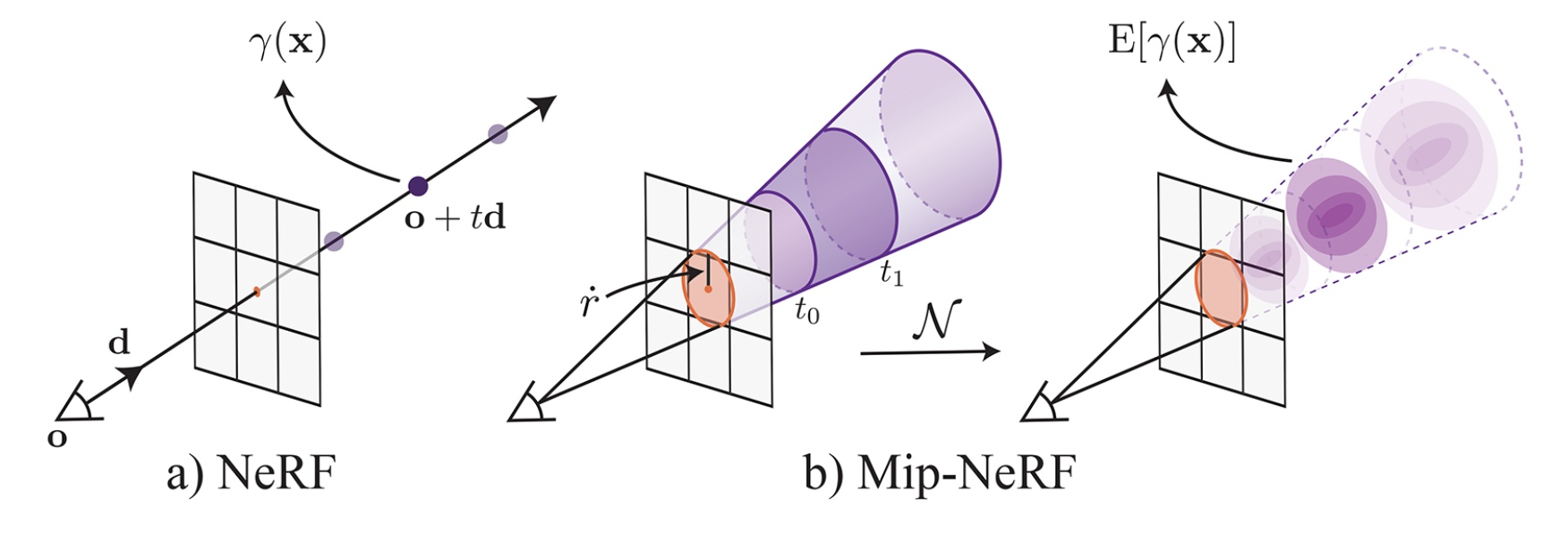
One technique worth highlighting is Integrated Positional Encoding (borrowed from Mip-NeRF). When rendering a pixel’s colour, standard NeRF treats a position as a point sampled from a beam of traced ray. Such setting makes NeRF unaware of its distance from the viewpoint because the same point yields the same feature no matter where you look at it. The consequence is a degraded rendering quality when NeRF has to render views in a wide range of scales (e.g. extreme close/ distant shot of the scene).
Instead of treating position as a point from a beam of ray, we can treat it as a conical frustum from a cone of rays. As a result, the network can reason about the distance of a position from the viewpoint based on the shape and size of the conical frustum. The same position traced from a further viewpoint should yield a larger conical frustum, illustrated below:
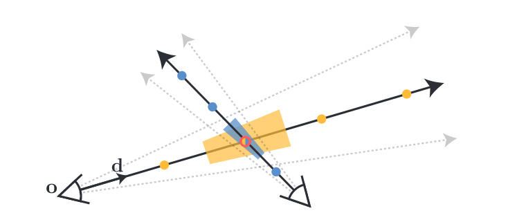
Such reframing implies that we have to treat $\bold{x}$ as a sample randomly drawn from a distribution resembling the conical frustum. Simulate $\bold{x}$ probabilistically would make the computation intractable, so we can featurize $\bold{x}$ by its expectation instead. To further simplify the setting, we can approximate ithe ill-shaped volumetric distribution by a nice-shaped multivariate Gaussian distribution. Such approximatation gives us a closed form on expected $\bold{x}$ transformed by positional encoding, aka $\mathbb{E}(\gamma(\bold{x}))$.
2.1.2. Colour Prediction by $f_{\bold{c}}$
The 2nd sub-network $f_{\bold{c}}$ predicts the RGB colour. Unlike density, colour requires more than position to describe. Here I list out factors that $f_{\bold{c}}$ considers:
Factor 1: Spatial Position
It is trivial to say that a scene has different colours at different positions. We make use of the embedding emitted from $f_{\sigma}$ to featurise this spatial information. As a recap of $f_{\sigma}$, the embedding featurises the position as a volume instead of a point, so $f_{\bold{c}}$ shares the same advantage as $f_{\sigma}$ to be aware of its distance from the viewer.
Factor 2: Viewing Direction
Depending on light source, an object’s surface has different brightness at different angles, hence difference in colours. We can tell a surface’s brightness from its illuminance - a technical term to measure the amount of lights spreading over a surface area. We can use unit vector $\bold{d}$ to capture the direction where we look at a point.
Factor 3: Exposure Level of a Camera
Exposure describes the amount of lights exposed to a camera’s film. High exposure leads to a bright view while low exposure leads to a dim view. Below diagram contrasts the same view at different exposure levels:
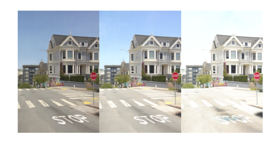
Exposure level is mainly controlled by shutter speed - a measurement of time when camera’s shutter opens for light to come in. High shutter speed captures sparse light and results in sharp image, while low shutter speed captures dense lights and results in blurry motion. Training images are collected in the wild so it is subject to a wide range of exposure levels. Conditioning $f_{\bold{c}}$ on exposure level helps it account for the variation.
BlockNeRF parameterises exposure level by shutter speed and 2 additional scaling factors: analog gain and $t$. It is further transformed by positional encoding with 4 levels, i.e. $\gamma_{4}(.)$.
Factor 4: Environmetal and Photometric Variations
Besides exposure level, training images are also subject to environmental variations (e.g. change in day of time/ weather) and photometric variations (e.g. different photographic visual effects). These variations could break standard NeRF because we could have training images of different appearances even at the same viewpoint (e.g. imagine day view v.s. night view). Such inconsistency confuses standard NeRF because it assumes the scene is static and controlled so same viewpoint should lead to same appearance
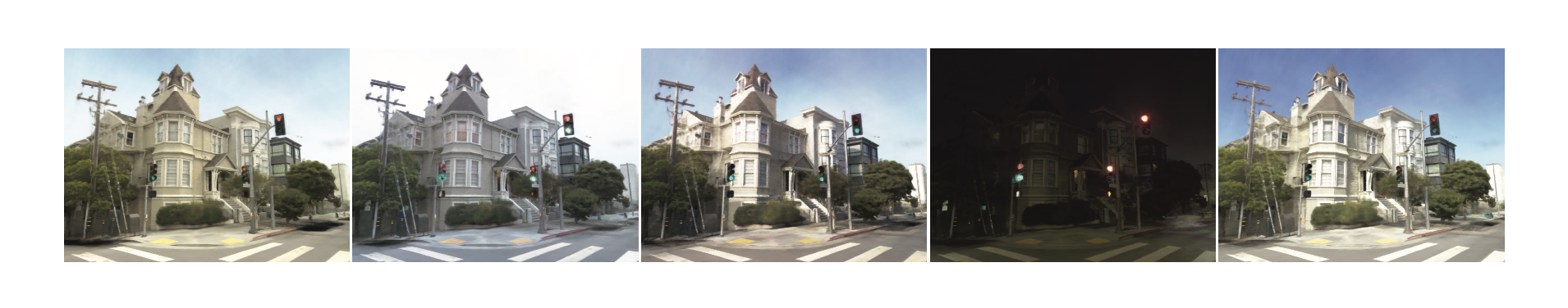
Therefore, the authors apply a technique called Appearance Embedding (borrowed from NeRF in the Wild). They introduce an auxiliary latent vector as an input to the network in order to describe the variations. Each image is assigned a latent vector and it helps explain away the variation of appearance specific to the image. Once learned, we can render novel views with any of these latent vectors to control appearance. Want to render a novel view with a night view like image A? Just append its associated latent vector when rendering!
The latent vectors are optimised alongside with the network through a technique called Generative Latent Optimization. You can treat it as an additional optimisation independently applied on each latent vector, with an objective to minimise the reconstruction loss against its associated image.
2.2. Visibility Prediction by $f_{v}$
Besides blocks of NeRF, we have a visibility network $f_v$ to holistically scan through the scene. It is inefficient to query all blocks when rendering, so visibility network helps filter blocks that gives material contributions. It evaluates how visible a place is from a viewpoint. If most places of the block are not visible from the viewpoint, then we can safely discard the block for rendering.
We could quantify the visibility of a place by its transmittance. It tells the chance of a ray passing from a viewpoint to the place. The densities along the way influence the transmittance because the ray may get blocked during its travel. Transmittance of close to 1 means high transparency along the way, close to 0 means it is likely blocked by solid particles along the way.
How to compute transmittance with the visibility network? Let’s say we are at position $\bold{o}$ viewing at direction $\bold{d}$, we can march a ray from our viewpoint and parameterise it as $\bold{r}(t) = \bold{o} + t \bold{d}$, where $t$ describes the distance from the viewpoint. Then we can collect discrete samples along distances $\{ t_k \}_{k=1}^{N}$ and evaluate their respective densities $\{ \sigma_k \}_{k=1}^{N}$ with the visibility network. With the quantities, we can numerically approximate the transmittance at distance $t_{i}$ by:
Compared against $f_{\sigma}$ and $f_{\bold{c}}$, visibility network $f_{v}$ is light-weight to efficiently query across blocks. It deploys the same Integrated Positional Encoding trick to capture positional information.
2.3. Masking Out Transient Objects
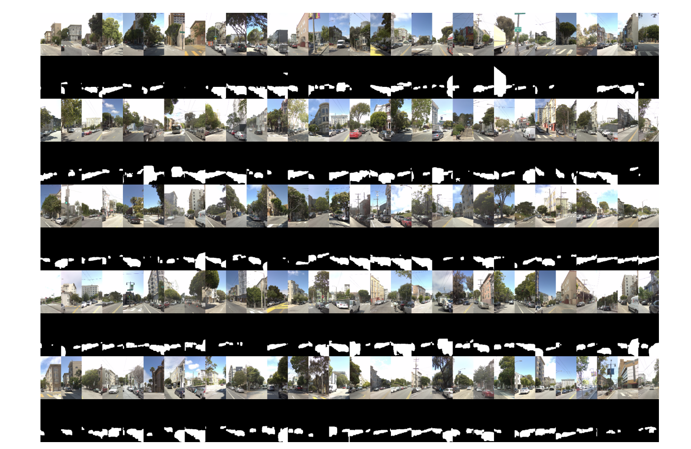
BlockNeRF targets to model the static landscape of the scene, but transient objects (e.g. pedestrians/ vehicles) in the training images obstruct its learning because their presence leads to view inconsistency. Below are examples where the same landmark have different groups of pedestrians at different time.
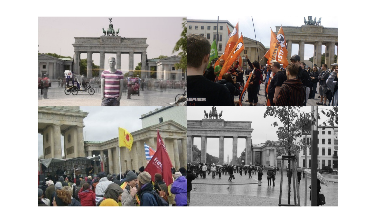
To address transient objects, we could bound their belonging regions with a pretrained semantic segmentation model, and then exclude the regions from the supervision. Recall that NeRF is supervised by minimising reconstruction loss between ground-truth pixels and rendered ones. Removing pixels associated to transient objects help eliminate inconsistent signals to NeRF.
3. Orchestrating the Blocks
3.1. Composing Blocks for Rendering
Once trained, we can render any novel view with the blocks. The simplest way to render a view during inference is to look at the block nearest to the viewpoint. However, the paper shows such naive approach leads to temporal inconsistency when animating a driving views across blocks. It creates abrupt jump in appearance upon block transition.
To make the views more consistent, we can blend the views rendered by several blocks. Doing so is computationally expensive so we can apply simple heuristics to filter relevant blocks. One simple rule is to scope the blocks within a fixed radius of the viewpoint. On top of that, we utilise visibility network $f_{v}$ to assess the overall contributions of each scoped block. We remove the block from final rendering if its average visibility (measured by transmittance) is below a certain threshold.
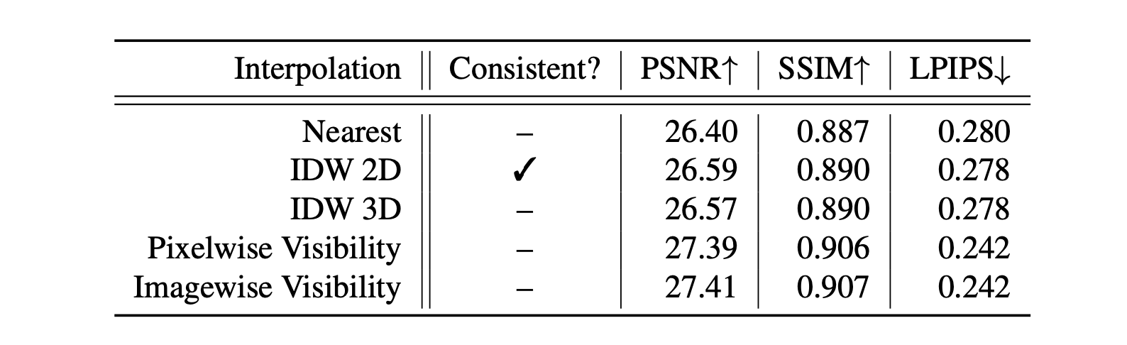
After these 2 simple filtering, 1-3 blocks remain for final blending. We can blend them together by interpolation. We use inverse distance weighting to determine the weight of each view:
$c$ is the viewpoint’s coordinate and $x_{i}$ is the coordinate of the block’s center. $p$ is a paramter that controls the rate of blending. The authors experimented different distance measures and interpolation methods. They conclude that 2D Inverse Distance Weighting (IDW 2D) yields that best results in terms of temporal consistency.
3.2. Aligning Appearance Across Blocks
We know we have to blend views from different blocks for rendering, but a key detail is missing: How do the views align their appearance? This is tricky because the blocks don’t share any agreement on how to decode the latent vector into appearance. Different blocks can decode the same latent vector as different appearances.
To address this, we performs an additional optimisation to enforce the consistency of appearance across blocks. Let’s say we want to render a views with a target appearance seen in a training image, we can retrieve its associated latent vector (target latent vector) from one of the responsible blocks (target block). With the target block and target latent vector, we can do the following:
- Freeze the target latent vector and network weights of all blocks
- Select a block adjacent to the target block
- Retrieve a latent vector for the adjacent block
- Render a view at a place commonly seen by both target block and the adjacent block
- Optimise the latent vector to close the difference between the view rendered by target block v.s. the adjacent block
Note that the paper doesn’t mention how the adject block retrieves a latent vector for optimisation. My educated guess is that it works either by randomly sampling one from its learned latent vectors or initialising from scratch. Regardless of how it is retrieved, it will eventually converge towards the target appearance. And the optimisation should be fast because we only need to optimise a latent vector.
At the beginning of the optimisation, we could expect the same view rendered by the 2 blocks have different appearances. But over the optimisation, the view rendered by the adjacent block will converge towards the target appearance, illustrated below:
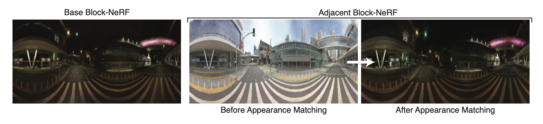
After that, we can propagate the same scheme of optimisation outward to other blocks. At the end all blocks have a latent vector responsible for the target appearance. Despite a perfect alignment is hard to achieve, this solution should preserve consistency on most macro attributes of the scene.
To make the above proposal work, each block has to overlap with its neighbours. The authors configure the blocks so that any 2 adjacent blocks have at least 50% overlap.
4. Results
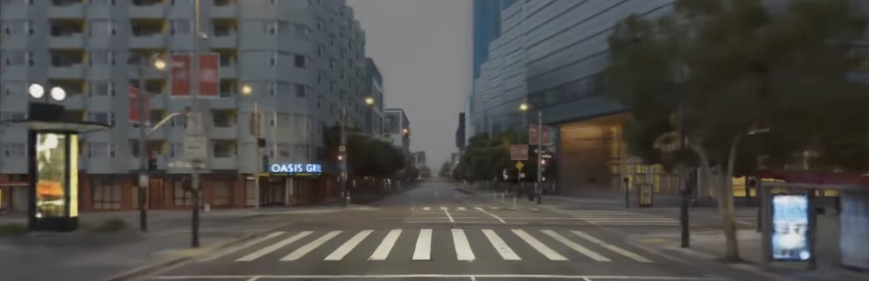
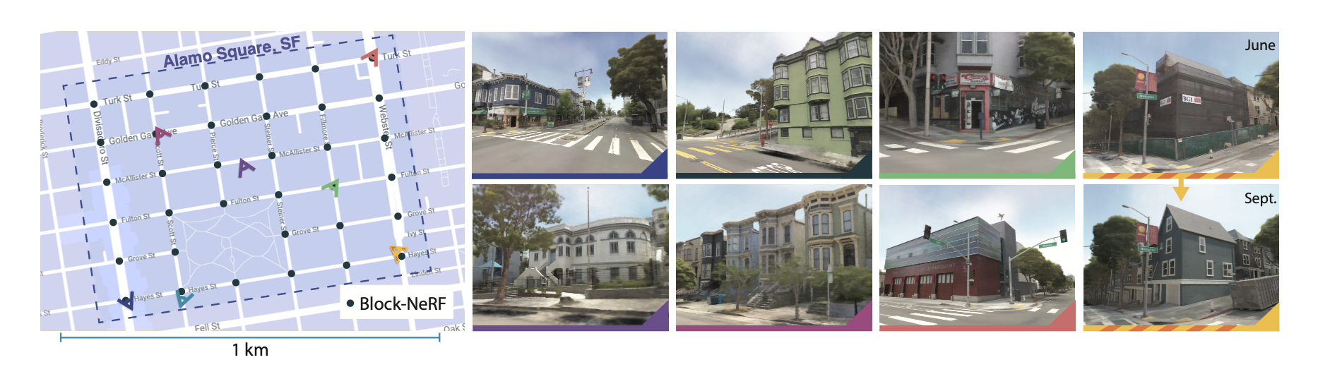
To showcase the power of BlockNeRF, the authors train BlockNeRF on 2.8 million posed images captured in San Francisco. They are collected on public roads with data collection vehicles from June 2021 to August 2021.
Since the training datasets are driving views collected by vehicles, so this work focuses on rendering novel driving views. The picture below cherry-picks the rendered views of different driving locations at Alamo Square (San Francisco). The pair of views on the right shows the modularity of BlockNeRF. There was a construction work undergoing on June 2021, which was completed at September 2021. If we want to update the scene with the renovated building, we only need to retrain the responsible blocks without the need to train all blocks again.
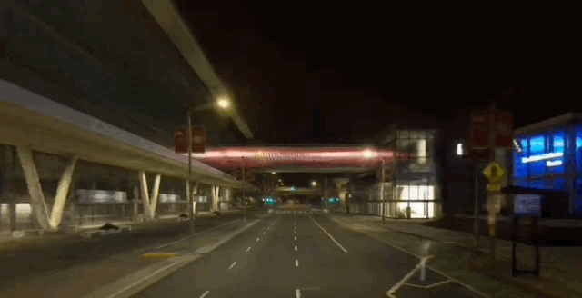
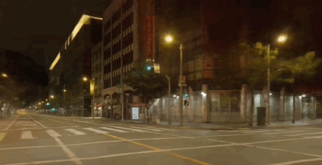
Here BlockNeRF animates a driving view at Moscone Center (San Francisco). You can see the night view smoothly transits to the day view thanks to the interpolation of their respective latent vectors.
Below is the same trick. BlockNeRF transits Downtown (San Francisco) from dawn to morning by interpolation of the learned appearance embeddings.
BlockNeRF can offer diverse driving scenarios because it is easily extensible and you can control both the exposure level and the appearance of a scene from model inputs.
5. Limitations
The authors list out some limitations of their work at the end. Here I highlight a few:
- Heavy computational footprint due to large scale training, hence the carbon emissions
- Inability to model dynamic scenes, solving which could unlease NeRF application on robotics
- Background is rendered blurry because limited blocks are used after filtering and they don’t cover most background
- Slow rendering speed and long training time, issues that other NeRF variants commonly suffer
6. References
- CSC2547 NeRF in the Wild Neural Radiance Fields for Unconstrained Photo Collections
- Mip-NeRF: A Multiscale Representation for Anti-Aliasing Neural Radiance Fields
- Block-NeRF: Scalable Large Scene Neural View Synthesis
- NeRF in the Wild: Neural Radiance Fields for Unconstrained Photo Collections
- Mip-NeRF: A Multiscale Representation for Anti-Aliasing Neural Radiance Fields
- INeRF: Inverting Neural Radiance Fields for Pose Estimation
- Optimizing the Latent Space of Generative Networks