Paper Summary: “MVSNet: Depth Inference for Unstructured Multi-view Stereo”

1. Motivations
2. Intuition of Plane Sweeping Stereo
3. Feature Extraction and Feature Map Warping
- 3.1. 2D CNN $f_{\bold{F}}$ for Feature Extraction
- 3.2. Differential Homography Applied on Feature Maps
4. Cost Volume and Probability Volume
- 4.1. Constructing Cost Volume $\bold{C}$
- 4.2. Constructing Probability Volume $\bold{P}$
5. Loss Function
6. Results
7. References

cover

1. Motivations

Multi-view stereo is a general technique of 3D scene reconstruction by associating correspondence between multiple views. Views from the same scene typically share high degree of content. We can leverage the point-wise associations between views to recover the 3D points of the shared content.

There are different approaches to find the correspondences. One classical approach is plane sweeping stereo. It esimates per-view depth map, and then jointly utilised the depth maps to estimate the 3D point clouds. This approach is scalable because it can process each view independently with low memory footprint. Despite its scalability, it struggles to recover challenging scenarios, such as region with occlusion, or surface that are specular or low-textured. It is hard to find correspondences of these regions using hand-crafted features. This issue could lead to noisy estimation of depth map.

To address the issue, the authors proposes MVSNet: an end-to-end deep learning pipeline resembling traditional sweeping plane approach. It is as scalable as traditional sweeping plane approach, with more robust depth map estimation.

from AI Labs.tw

2. Intuition of Plane Sweeping Stereo

Before diving into MVSNet’s pipeline, let’s have a quick look of how plane sweeping stereo works. Understanding its key idea helps understand the basis that MVSNet is built upon.

The objective is to estimate a depth map for a view. Let’s call the view as reference view $\bold{I}_{1}$ and denote the other views as source views $\{ \bold{I}_{k} \}_{k=2}^N$. The algorithm makes use of all $N$ views (both reference view and source views) to do the estimation.

Imagine you insert a suite of virtual planes into the scene that are parallel to the reference view. Let’s say there are $D$ of them. These planes are uniformly apart with varying distance from the reference view. These planes represent different hypotheses of depth values.

Next, we cast a viewing frustum of the reference camera into the scene. Following the frustum we project the reference view into each virtual plane. We end up with $D$ projections, essentially different enlargment of the reference view.

For the rest of the views, we can warp each of them into each virtual plane, at the same place where the reference view is projected. Since we know camera matrix of each view, we can apply classical homography to warp a source view to the target projection, and then express its image coordinate with respect to reference camera.

After warping all views, we should have $N$ warped images on each plane. We can then evaluate the pixel-wise variance across the $N$ warped images. The intuition is to estimate how likely the $N$ warped images are projecting the same content at the same pixel position. Low variance indicates the 3D point associated to the target pixel is likely to lie on that plane. Therefore, we can estimate the depth of the target pixel by the depth of that plane.

The above procedures can be visualized by the following diagram. For simplicity, we use colour as a naive feature. Notice the target pixel has the lowest variance in colour at the second plane, so its associated depth $d_{2}$ is the best estimate of target pixel’s depth.

from Fall 2021 CS 543/ECE 549: Computer Vision

Note: Since this session aims to offer high-level intuition, I skipped its technical details. Also for the diagram above, I use colour as feature but it is usually not favorable because it is vulnerable to variations like illuminance difference.

3. Feature Extraction and Feature Map Warping

3.1. 2D CNN $f_{\bold{F}}$ for Feature Extraction

MVSNet’s pipeline is basically similar to plan sweeping stereo, except it swaps in learnable components into a few places.

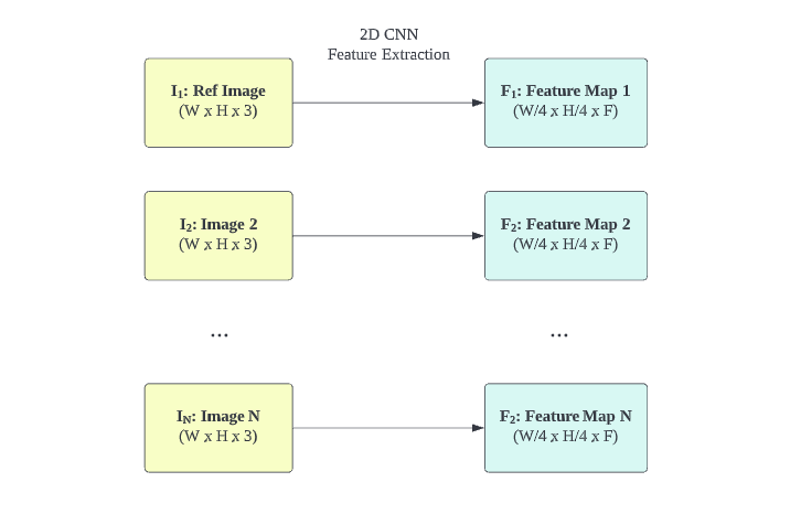
Knowing that hand-crafted feature is not robust to diverse variations, MVSNet deploys a learnable 2D Convolutional Neural Network (CNN) $f_{\bold{F}}$ to extract features from each view. The extracted features should capture rich local semantics, so it is more robust to different variations.

f_{\bold{F}}(\bold{I_{i}}) = \bold{F_{i}}

Let’s say a view $\bold{I_{i}}$ has a dimension of $(W \times H \times 3)$ including RGB channel. The CNN returns its downsampled feature map $\bold{F_{i}}$ of dimension $(W/4 \times H/4 \times F)$, with $F$ being the size of feature channel. $f_{\bold{F}}$ serves as a feature extractor. It transforms a set of views $\{ \bold{I}_{k} \}_{i=1}^{N}$ into a set of feature maps $\{ \bold{F}_{k} \}_{i=1}^{N}$, visualized as follows.

3.2. Differential Homography Applied on Feature Maps

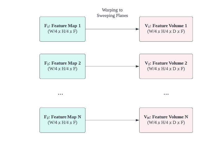
By the principle of homography, we can warp feature maps to each sweeping plane in front of the reference view.

Since the homography transformation is just a matrix multiplication with a feature map, it is differentiable and can be backpropagated. Such nice property makes homography transformation integrable into the end-to-end pipeline. This enables MVSNet to be aware of geometric relationships between different views, so as to learn the 3D geometry of the scene.

A set of feature maps $\{ \bold{F}_{k} \}_{i=1}^{N}$ of dimension $(W/4 \times H/4 \times F)$ are warped to a set of feature volumes $\{ \bold{V}_{k} \}_{i=1}^{N}$ of dimension $(W/4 \times H/4 \times D \times F)$.

4. Cost Volume and Probability Volume

4.1. Constructing Cost Volume $\bold{C}$

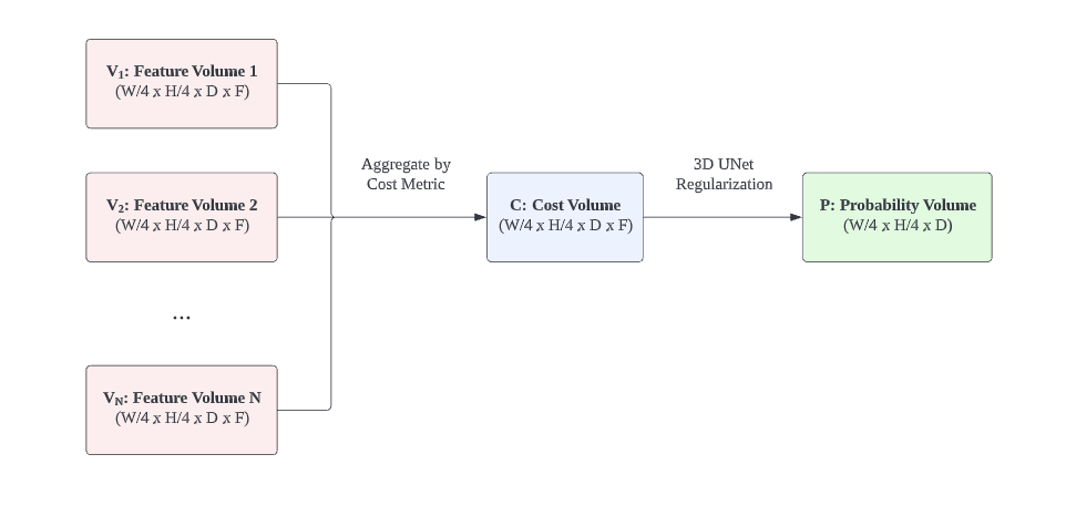
Now we need to aggregate the set of feature volumes $\{ \bold{V}_{k} \}_{i=1}^{N}$ into a single tensor. This is tricky because the number of views $N$ is arbitrary.

The authors propose variance-based metric to reduce the feature volumes set into a tensor of dimension $(W/4 \times H/4 \times D \times F)$. The metric is essentially an element-wise variance across feature volumes. The variance-based metric is in line with the principle of traditional plane sweeping stereo. It measures multi=feature consistency at different pixel position at different depth.

The tensor it returns is called Cost Volume $\bold{C}$.

\bold{C} = \text{Var}(\bold{V_{1}},...,\bold{V_{N}}) = \frac{\sum_{i=1}^{N} (\bold{V_{i}} - \bold{\bar{V})^2}} {N}

Here $\bold{\bar{V}}$ is the element-wise average of $\{ \bold{V}_{k} \}_{i=1}^{N}$ and the whole operation is differentiable.

4.2. Constructing Probability Volume $\bold{P}$

Notice the Cost Volume encodes multi-feature consistency in its $F$ channel. It is hard to infer depth based on those high-dimensional quantities.

In addition, the Cost Volume is especially noisy on regions with occlusion or tricky surface. To make the subsequent depth estimate more accurate, we can apply smoothing on the Cost Volume. It could effectively smooth away noise based on information from its neighboring pixels.

To this end, the authors introduce a learnable 3D CNN UNet $f_{\bold{P}}$ to transform the Cost Volume into a tensor of dimension $(W/4 \times H/4 \times D)$. It serves to aggregates $D$ channel and smooth away the noise from the Cost Volume.

f_{\bold{P}}(\bold{C}) = \bold{P}

The last layer is a softmax applied on $D$ channel, so the resultant tensor is a Probability Volume $\bold{P}$ which expresses the pixel-wise depth as a probability distribution. You can treat the pixel-wise depth estimation as a classification problem. The probability distribution signals which sweeping plane the associated 3D point is likely to lie on.

5. Loss Function

5.1. Initial Depth Map $\bold{D}_{i}$

Argmax (winner-take-all) is not differentiable so we shouldn’t use it to get the estimated depth map from Probability Volume.

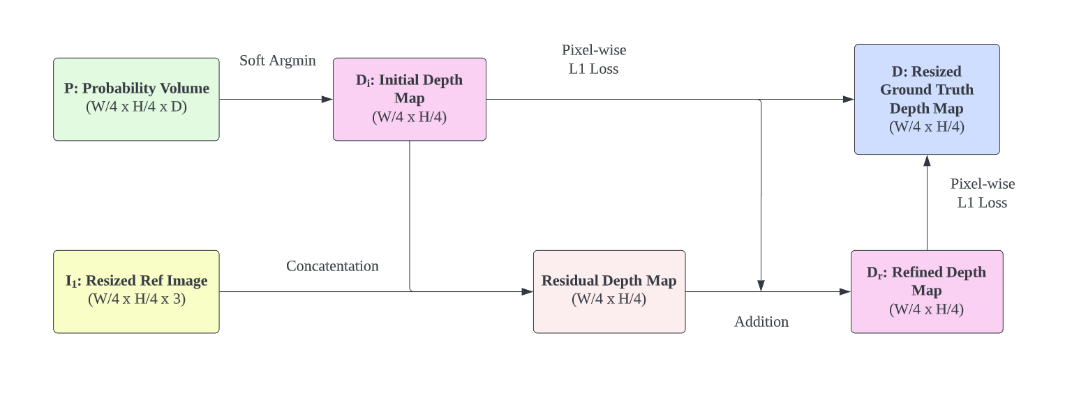
An alternative is Soft Argmin operation. It is no different from a pixel-wise expectation over the probability distribution of its depth. We can estimate the initial depth map $\bold{D_{i}}$ with soft argmin operation. Its dimension is $(W/4 \times H/4)$.

The predicted depth at pixel position $(u, v)$ is:

\bold{D}_{i}(u, v) = \sum_{d=d_{min}}^{d_{max}} d \times \bold{P}(u, v, d)

$d_{min}$ and $d_{max}$ is the depth of the closest and furthest sweeping plane, while $\bold{P}(u, v, d)$ is the probability that pixel position $(u, v)$ has a depth of $d$.

5.2. Refined Depth Map $\bold{D}_{r}$

Initial depth map may suffer from over-smoothing on its boundary caused by the 3D CNN UNet.

To address this, the authors introduce a 2D CNN $f_{r}$ to predict a residual map from the initial depth map $\bold{D_{i}}$ and the resized reference image $\bold{\tilde{I}}_{1}$. $\bold{D}_{i}$ and $\bold{\tilde{I}}_{1}$ are concatenated before feeding to network.

Composing the residual and the initial depth map gives a refined depth map $\bold{D}_{r}$:

f_{r}(\bold{D}_{i}, \bold{\tilde{I}}_{1}) + \bold{D}_{i} = \bold{D}_{r}

5.3. Putting Them Together as Supervision

To complete the training pipeline, we compare the ground truth depth map against both the initial depth map and the refined depth map.

All 3 networks $f_{\bold{F}}$, $f_{\bold{P}}$, $f_{r}$ are learned to minimise the absolute differences.

6. Results

Once MVSNet is trained, you can deploy it to estimate the depth map for a view.

The inference pipeline works the same as training one. You treat the view of interest as a reference view, and then warp all views onto its associated sweeping planes. You feed them to the trained MVSNet, and it runs through the pipeline to give you its estimated depth map. What makes it even more powerful is its capacity to generalize on unseen scenes. Even if the input views are from novel scenes, MVSNet is still able to reliably estimate their depth maps.

The authors propose an additional post-processing step to further filter the depth map.

After post-processing, MVSNet significantly outperform preceding models. The authors compare its reconstruction quality against different models for various scenes. It shows that preceding models fail to reconstruct a number of regions. In contrast, MVSNet managed to recover those regions.

The improvement can be attributed to the robust feature representation learned by $f_{\bold{F}}$. Additionally, $f_{\bold{P}}$ and $f_{r}$ (together with post-processing) further improve the quality of the predicted depth map.

Quantitatively, MVSNet outperforms preceding models by a large margin in most aspects, as shown: